Sorting 600 Curves by Z Value: Native Grasshopper vs. GHPython
Every Grasshopper user eventually hits the same fork in the road. Keep wiring native components together, or drop into a Python node. Here is what that decision actually looked like on a real 600 curve sort.
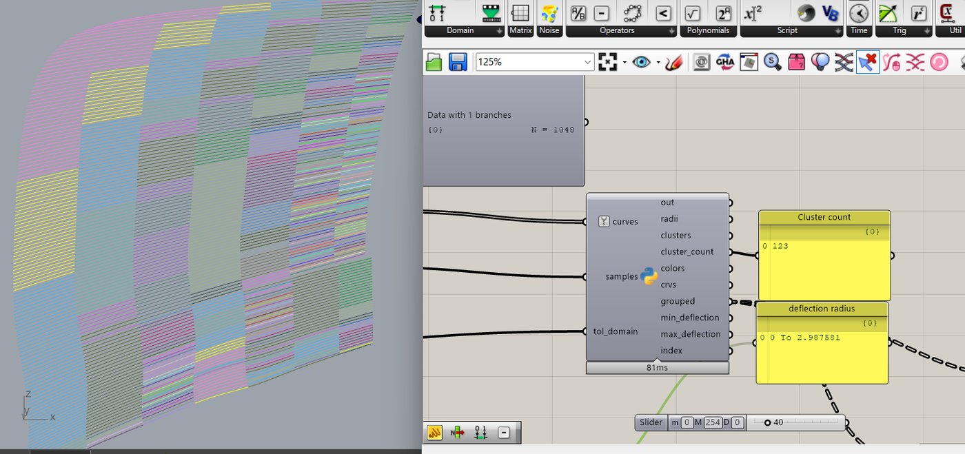
The actual GHPython component from a real sort-and-group script: curves and a tolerance in, cluster count and per-cluster colors out. 1,048 branches sorted and grouped in the viewport.
Sorting and grouping 600 curves by their Z value sounds like the kind of task Grasshopper's native components should handle without ceremony, and for a while, they do. The interesting part isn't whether it's possible natively. It is. It's at what point native components stop being the right tool, and why.
The native path
Native Grasshopper handles this cleanly with a small chain. Extract each curve's midpoint or a representative point, pull its Z coordinate, feed that list into a Sort component alongside the curve list as the values to sort, then group the sorted output using a Partition style pattern on the Z values, bucketing anything within a tolerance band into the same group. No code, fully visible on the canvas, easy for someone else to open the file and understand what's happening step by step.
Where it starts to strain
The strain shows up in three places as complexity grows. First, grouping by a tolerance band rather than an exact match doesn't have a single clean native component. It usually means chaining several list and culling components together in a way that works but is genuinely harder to read than the equivalent five lines of code. Second, anything conditional, group A unless condition X applies, in which case handle it differently, turns into an increasingly tangled wire diagram. Third, canvas performance. 600 curves through a dense native chain with multiple data tree operations is noticeably slower to solve than the same logic in one Python component, because each native component is its own solve step with its own tree matching overhead.
The GHPython version
The equivalent in a single GHPython component: extract Z values, pair them with their curves, sort the pairs, then run a simple tolerance based grouping loop.
pairs = sorted(zip(z_values, curves), key=lambda p: p[0])

groups = []
current_group = [pairs[0]]

for z, curve in pairs[1:]:
    if abs(z - current_group[-1][0]) <= tolerance:
        current_group.append((z, curve))
    else:
        groups.append(current_group)
        current_group = [(z, curve)]

groups.append(current_group)
This solves in one step instead of a chain of six or seven, and the tolerance grouping logic, the part that was awkward natively, comes down to three readable lines. The tradeoff is real too. It's a black box on the canvas. Anyone opening the file has to open the Python editor to see what it does, instead of reading it straight off wired components.
The actual decision rule
What settled it wasn't performance or line count. It was who else needs to open the file. For a one off internal script, GHPython won outright: faster to write, faster to solve, easier to modify. For anything meant to be handed to a junior team member or used as a teaching example, native components stayed the better choice even when clunkier, because the logic being visible on the canvas is worth more than the extra wires. The 600 curve sort itself ended up as a Python component. The simplified teaching version of the same workflow stayed native.